This page expands on some of the topics in PS #0, prob 2. Recall that we derived equations that described the following first order reaction,
A --> B.
The fraction A remaining after time, t, is
[A]/[Ao] = exp(-kt).
One way to evaluate k, the rate constant, is to take logarithms, yielding,
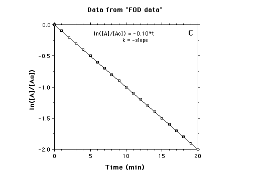
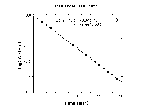
ln([A]/[Ao]) = - kt; alternatively, 2.303 x log([A]/[Ao]) = -kt.
A graph of the LHS vs t will give us k as the -slope.
First order decay simply means that for a population of atoms (e.g. radioactive), molecules (our example of A --> B), or anything else, a constant fraction/unit time is converted to something else. The actual fraction/unit time is expressed as k (the rate constant, in units of time
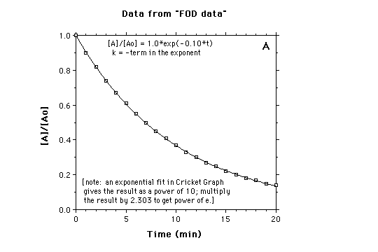
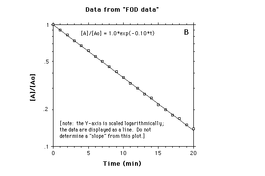
In the above example, if k = 0.10/min, then 10% of A at any time will be converted to B in the next one minute. The following four graphs show different ways of displaying first-order decay data. The values for [A]/[Ao] at the times indicated were calculated with k = 0.10 min
A. Plot of [A]/[Ao] vs time.
B. Plot of [A]/[Ao] vs time, with the Y-axis logarithmic.
C. Plot of ln([A]/[Ao]) vs time.
D. Plot of log([A]/[Ao]) vs time.
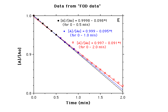
E. Plot of [A]/[Ao] vs time, for a short time interval.
Here we plot only the first portion of the reaction, with linear fits to the data. This approach is termed the "initial rate" method. Let's evaluate k from the slopes of these linear fits.
a) The "black data" correspond to the first 5% of the reaction. A linear fit yields k = 0.098 min
b) The "blue data" correspond to the first 10% of the reaction. A linear fit
yields k = 0.095 min![]() ,
about 5% lower than the true value of 0.10 min
,
about 5% lower than the true value of 0.10 min![]() .
.
c) The "red data" (first 20% of the reaction) give us k = 0.091 min![]() , about 9% too low.
, about 9% too low.
This example shows that an exponential curve (or any other curve) can be approximated by a straight line over small regions. However, it is usually best to confine linear fits of initial rate data to the first 5% or less of a first order decay curve. This limitation can be an advantage if we know that a very slow process is characterized by first order decay; then we can determine k without following the reaction for large fraction reactions, i.e. excessive times.
A given rate constant can be converted to any other units of time
The biochemistry and chemistry literature usually reports first-order rate constants in units of sec
Note that both of the above terms are expressed in units of time.
If you have the idea of first order decay under control, you should be able to solve the following problems (ideally, without recourse to graphs or equations) with a calculator.
Final comment: e, the base of natural logarithms, appears in all of the equations for first order decay (and in many other equations in science). A history of this curious number (2.718...) and a lucid description of simple calculus can be found in
Return to thePS #0 Graphs page. ![]() Back
to ABC98 Home Page
Back
to ABC98 Home Page